For the WGNSS Nature Photography Group’s January outing we headed to Carlyle Lake in Illinois. Our primary target was the dam’s spillway. I have had a lot of fun at this location photographing Bonaparte’s Gulls and American White Pelicans during past winters and these species are what we were hoping for on this trip.
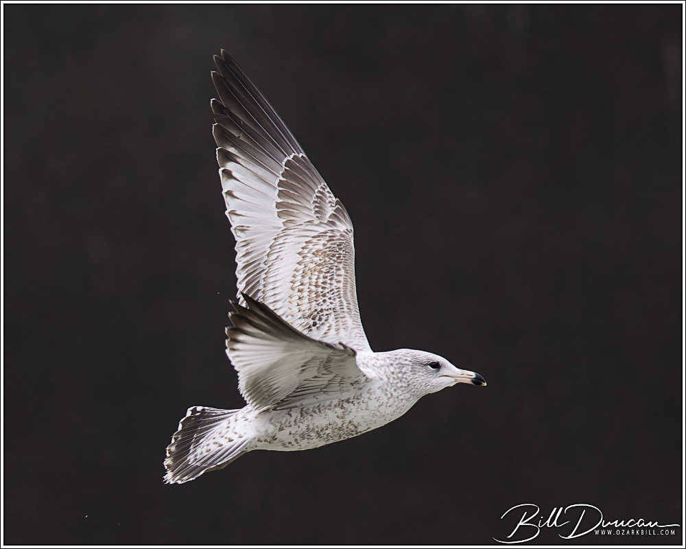
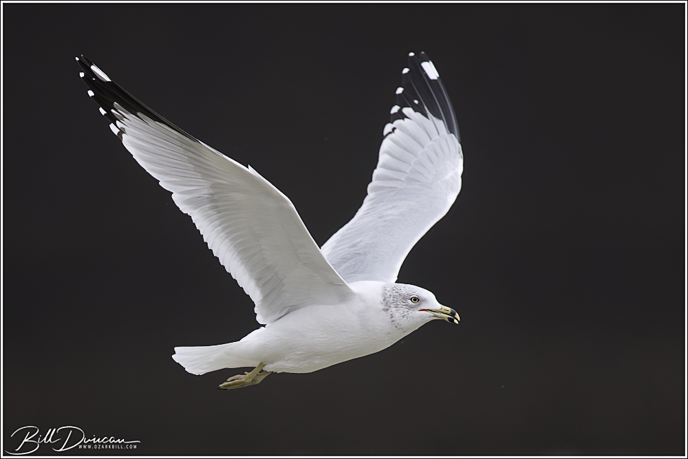
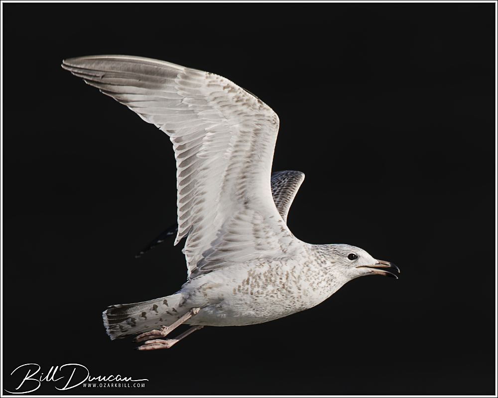
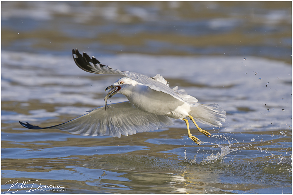
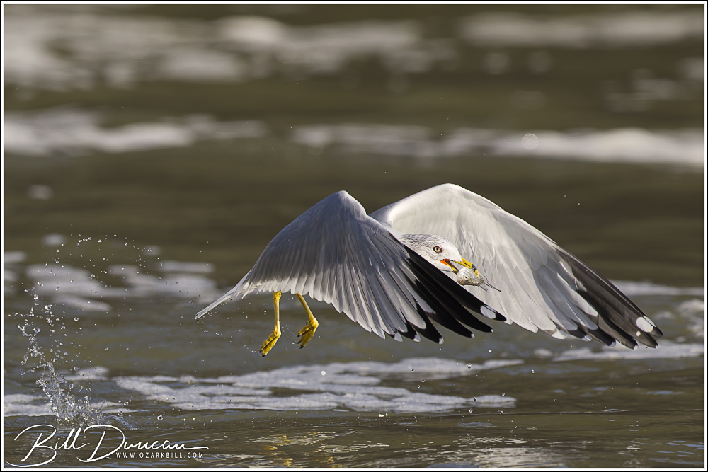
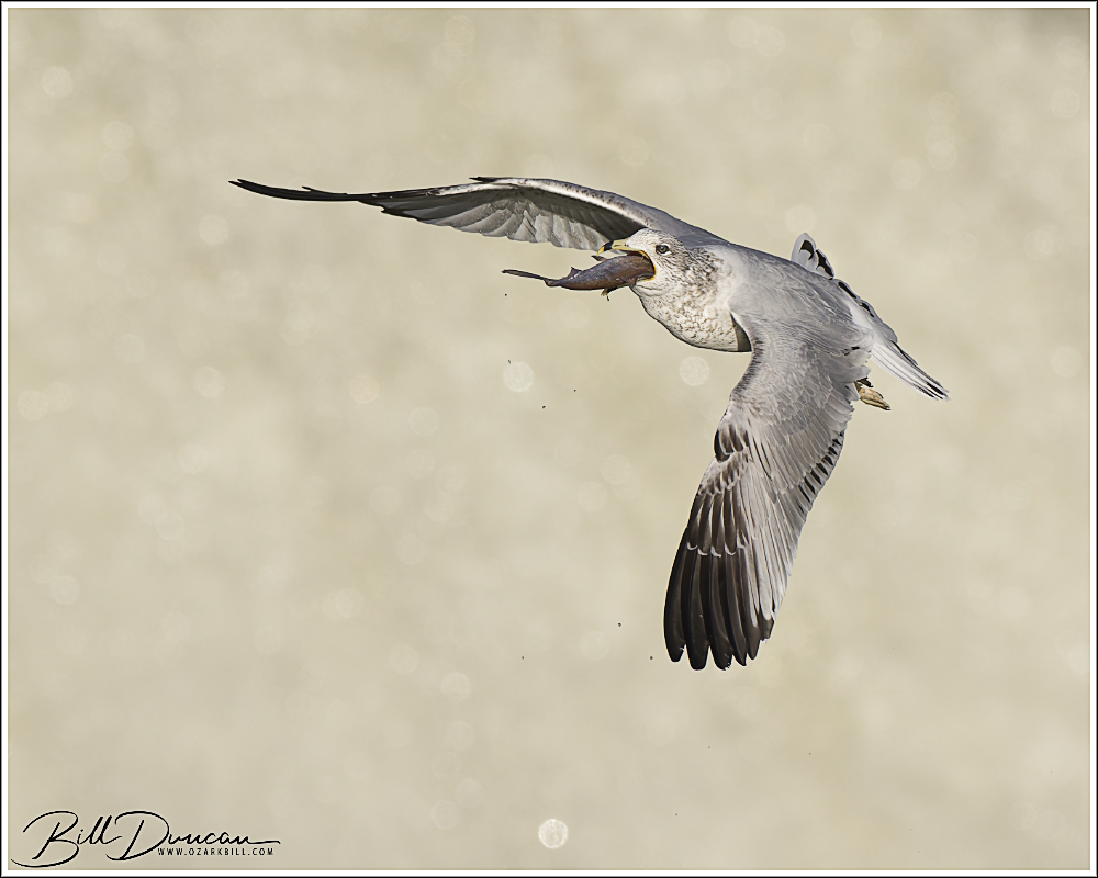
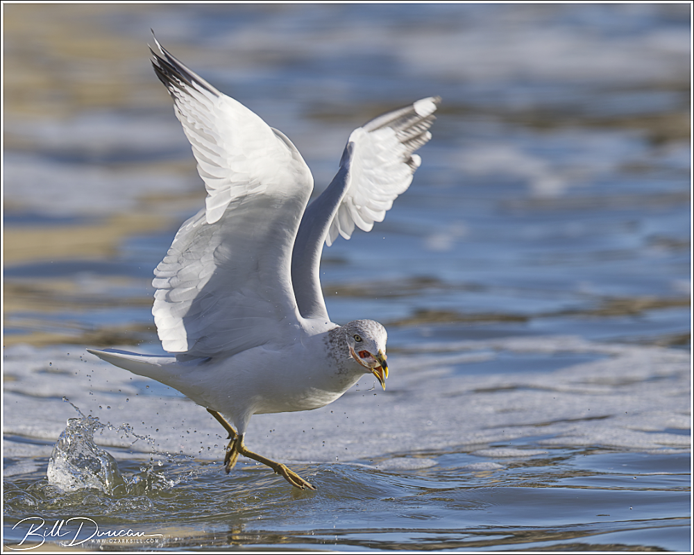
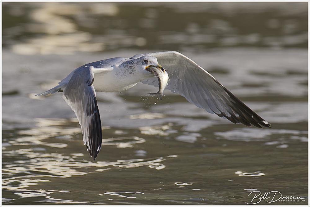
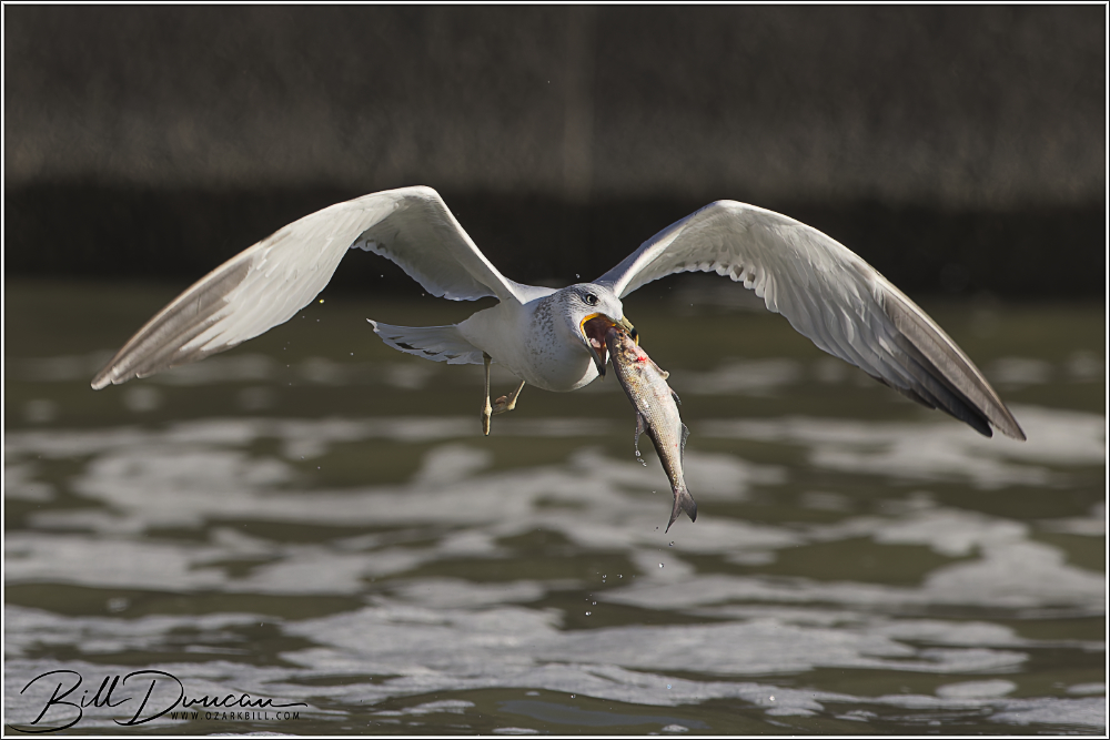
Being a spillway with the dam and infrastructure surrounding it, the backgrounds are definitely challenging; however, it is not impossible to handle. The images below showcase one method we could use to handle this situation. With the rising sun at our backs, I noticed the light was hitting these mostly white birds perfectly. By exposing precisely for the whites and a little exposure manipulation in post-processing, it was possible to turn the darker concrete walls of this section of the spillway nearly black, which allows the birds to pop off this background as seen in the images below.
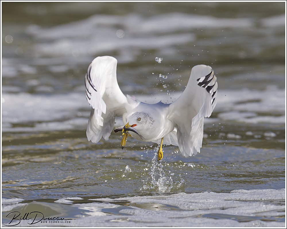
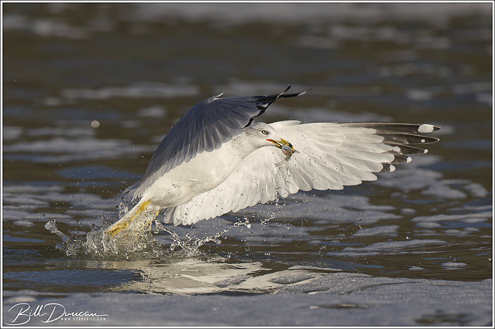
Predicting the movement of birds in a typical winter is difficult and this winter, where seasons have been changing on a daily basis, is pretty much impossible. On top of that, water levels in the lake and spillway channel were a couple feet below normal. The spillway gates were releasing just enough water, which I believe limited the numbers and size of fish falling through. So, it wasn’t surprising that we found almost nothing but Ringed-bill Gulls (RBGU) fishing in the spillway.
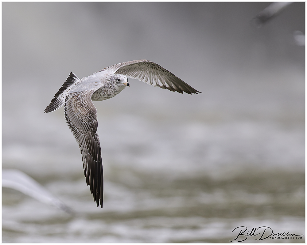
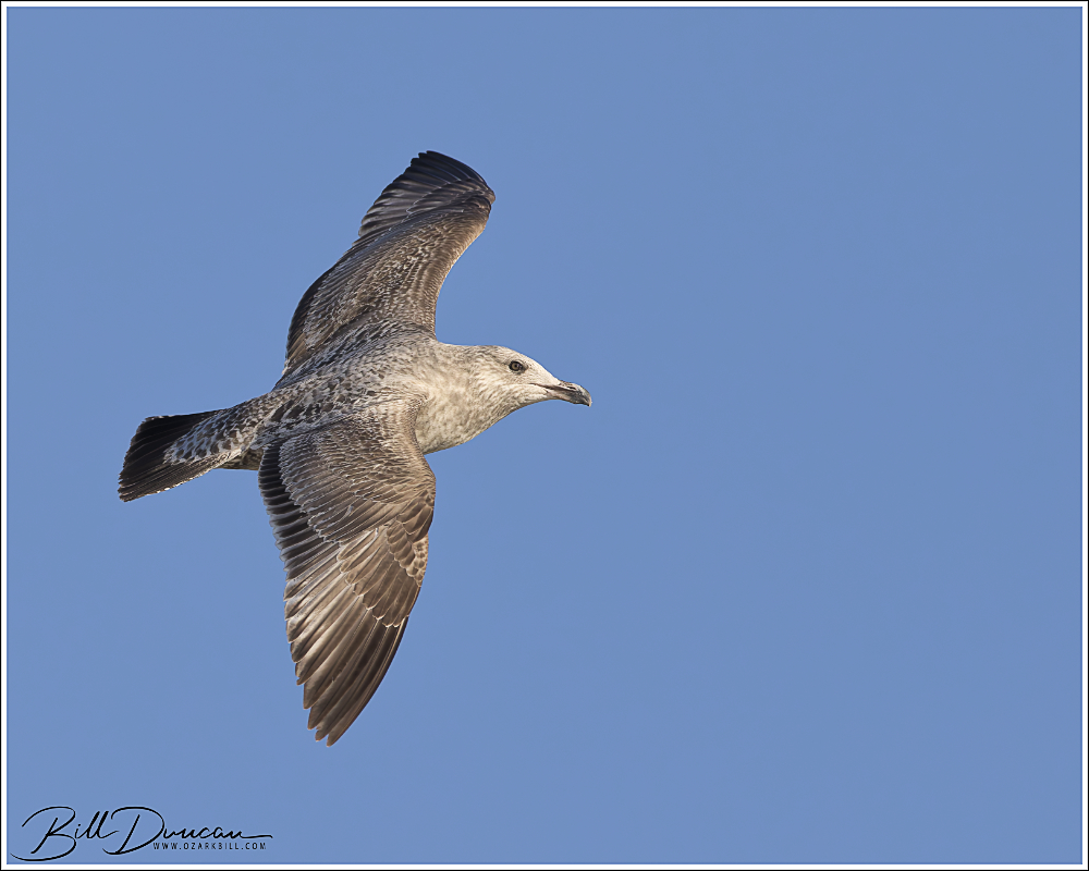
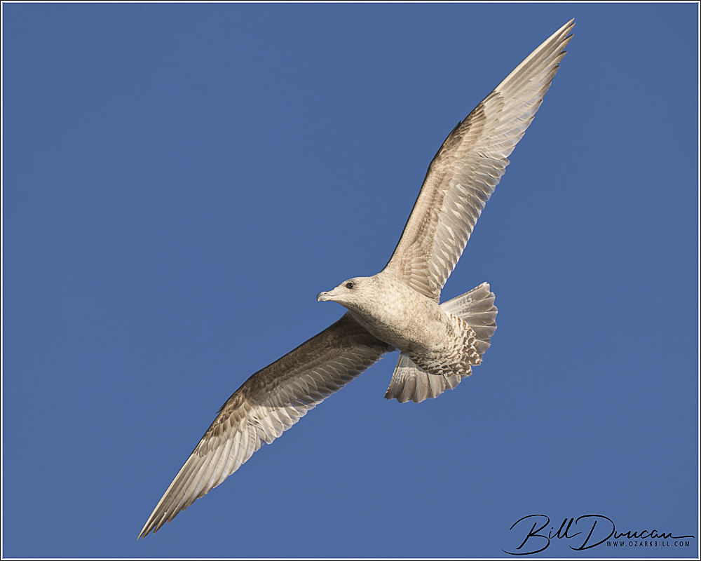
Ring-billed Gulls are considered 3-year gulls, meaning that they have a plumage transition for the first three years of their lives before they develop into the typical adult plumage. In addition, there is considerable variation within these years, e.g. a 2 year old gull may look different from a 2.5 year gull. Given I am no expert, I have made some captions with my best guesses on the ages of some of these birds.
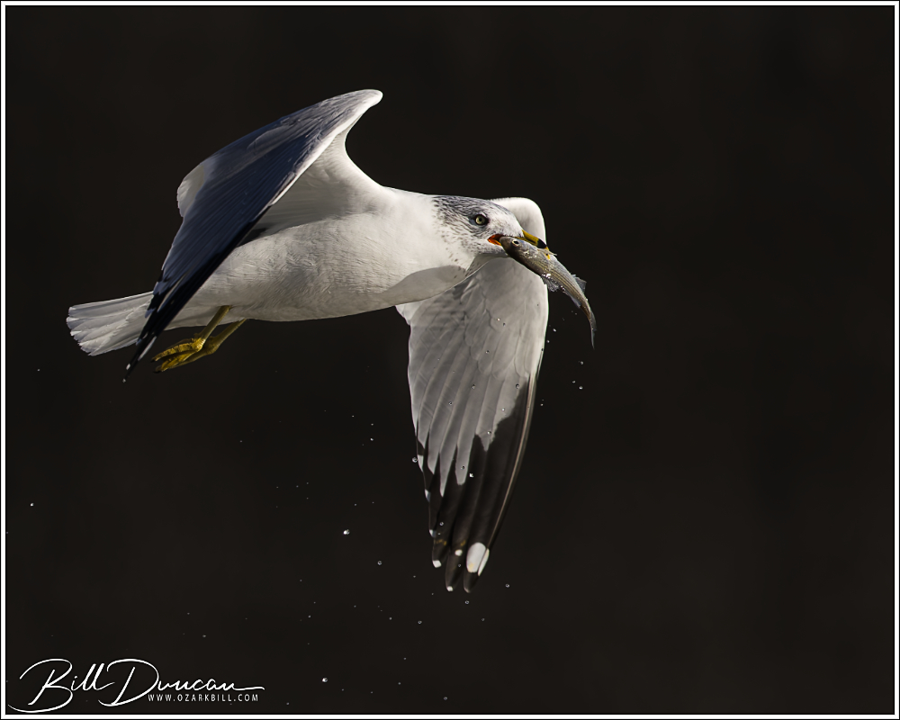
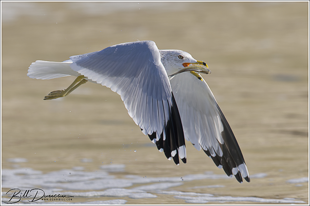
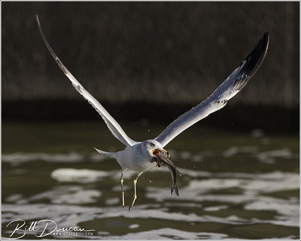
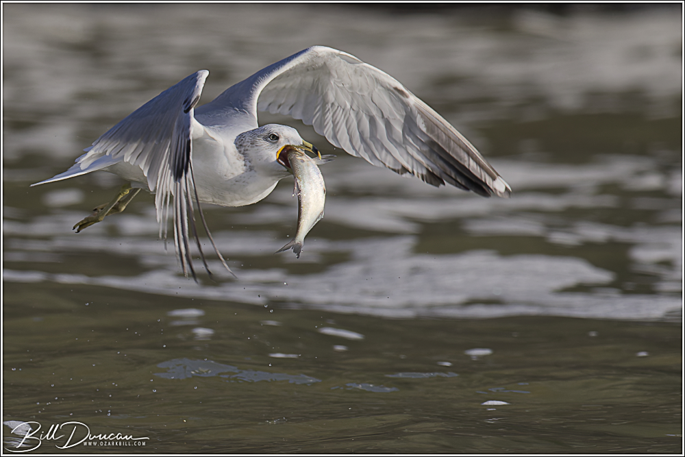
Another method of dealing with ugly backgrounds at this location is to focus on the fishing activities or other opportunities where the water will be the background of the image.
Many nature photographers would consider this a bust of a day and would perhaps head back home to watch a meaningless football game. However, I like to look at this as both an opportunity for practice and to potentially learn something new about a species taken for granted and usually ignored. I liken opportunities such as this to batting practice in three ways: 1) It gives you a chance to hone your skills – this is high-speed action photography with challenging backgrounds and dynamic lighting. If you haven’t mastered your camera’s exposure and autofocus settings, you will likely struggle getting the images you envision, 2) It’s a lot of fun! Whatever species you find in a spillway like this, there will likely by plenty of birds fishing, giving plenty of opportunities to capture those fleeting moments, and 3) with a species like the RBGU, you won’t likely come away with anything to brag about. These aren’t eagles or owls or some rare species that will be all the talk on social media.
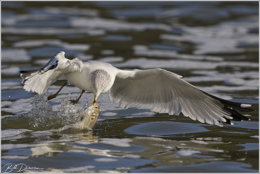
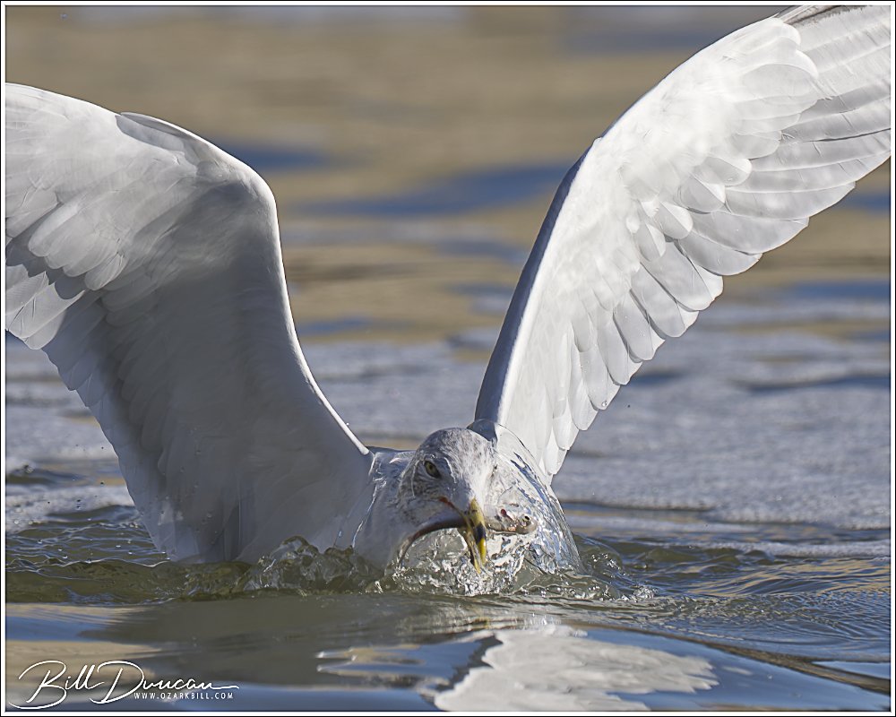
I really enjoyed watching the gulls catch and position their fish in flight for the head-first swallow. I was fortunate enough to catch this in action in several of my photos – they literally give them a little toss and catch them again so that the head is facing towards their mouth. It was also interesting to watch a few who knew the fish was too large to ingest and subsequently released back to the water.
As I alluded to above, I had a lot of fun shooting these gulls. The feeding opportunities were not as plentiful as I usually find at this location, but by staying alert and ready I came home with some photos that I really like.
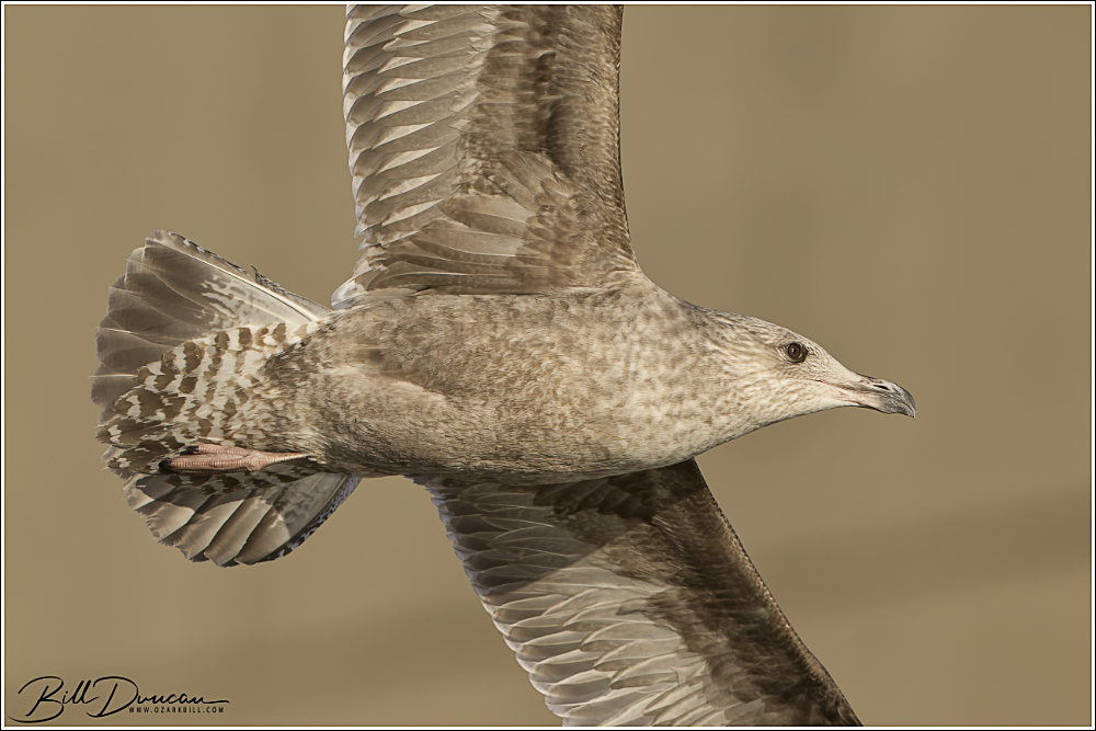
Ring-billed Gulls were not the sole fishers we found. We also had several first-year Herring Gulls shown below. Unfortunately these birds did none of their own fishing, but seemed content in attempting to steal the catch from the RBGU.
Thanks for visiting!
-OZB